Spline

Links

Finite Differenz

Die einfachste Methode zur Wahl der Tangenten ist die Verwendung der finiten Differenz. Mit ihr lassen sich die Tangenten für ein Segment im Einheitsintervall und 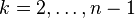$k = 2,\ldots,n-1$ wie folgt berechnen:

m_k \ = \ \frac{p_{k}-p_{k-1}}{2} + \frac{p_{k+1}-p_{k}}{2}

Für Endpunkte ( $k=0$ und $k=n$ ) wird entweder die einseitige Differenz verwendet, was effektiv einer Verdoppelung des Anfangs- und Endpunktes entspricht. Alternativ wird ein Vorgänger $p_{-1}$ und Nachfolger $p_{n+1}$ geschätzt, wofür es verschiedene Ansätze gibt.

Catmull-Rom-Spline

Tangente vom Catmull-Rom-Spline bei unterschiedlichem Faktor

T_1

Fasst man obige Gleichung zusammen, multipliziert sie mit 2 und definiert einen Faktor $T_k$ erhält man das Catmull-Rom-Spline.

\begin{align} {m}_k \ & = \ T_k (p_{k+1} - p_{k-1}) \ \text{mit} \ T_k \in [0,\infty) \qquad & \text{(Einheitsintervall)} \\ {m}_k \ & = \ T_k \frac{p_{k+1} - p_{k-1}}{x_{k+1} - x_{k-1}} \ \text{mit} \ T_k \in [0,\infty) \qquad & \text{(Werteintervall)} \end{align}

Aus dem Teilstück $p_{k+1} - p_{k-1}$ der Gleichung ist ersichtlich, dass die Tangente sich an der Richtung des Vektors von $p_{k-1}$ nach $p_{k+1}$ orientiert. Der Parameter $T_k$ skaliert unterdessen diesen Vektor, sodass das Kurvensegment weiter oder schärfer wird. Häufig wird dieser Parameter fest auf $0,5$ gesetzt, womit sich wieder die Ausgangsgleichung ergibt.

Benannt ist diese Kurve nach Edwin Catmull und Raphael Rom. In der Computergrafik wird diese Form häufig genutzt um zwischen Schlüsselbildern (Keyframes) zu interpolieren oder grafische Objekte darzustellen. Sie sind hauptsächlich wegen ihrer einfachen Berechnung verbreitet und erfüllen die Bedingung, dass jedes Schlüsselbild exakt erreicht wird, während die Bewegung sich weich und ohne Sprünge von Segment zu Segment fortsetzt. Dabei ist zu beachten, dass durch die Änderung eines Kontrollpunktes sich über die Bestimmung der benachbarten Tangenten insgesamt vier Kurvensegmente verändern.

Quelle: http://paulbourke.net/geometry/

Interpolation methods

Written by Paul Bourke
December 1999

Discussed here are a number of interpolation methods, this is by no means an exhaustive list but the methods shown tend to be those in common use in computer graphics. The main attributes is that they are easy to compute and are stable. Interpolation as used here is different to "smoothing", the techniques discussed here have the characteristic that the estimated curve passes through all the given points. The idea is that the points are in some sense correct and lie on an underlying but unknown curve, the problem is to be able to estimate the values of the curve at any position between the known points.

Linear interpolation is the simplest method of getting values at positions in between the data points. The points are simply joined by straight line segments. Each segment (bounded by two data points) can be interpolated independently. The parameter mu defines where to estimate the value on the interpolated line, it is 0 at the first point and 1 and the second point. For interpolated values between the two points mu ranges between 0 and 1. Values of mu outside this range result in extrapolation. This convention is followed for all the subsequent methods below. As with subsequent more interesting methods, a snippet of plain C code will server to describe the mathematics.

double LinearInterpolate(
   double y1,double y2,
   double mu)
{
   return(y1*(1-mu)+y2*mu);
}

Linear interpolation results in discontinuities at each point. Often a smoother interpolating function is desirable, perhaps the simplest is cosine interpolation. A suitable orientated piece of a cosine function serves to provide a smooth transition between adjacent segments.

Cubic interpolation is the simplest method that offers true continuity between the segments. As such it requires more than just the two endpoints of the segment but also the two points on either side of them. So the function requires 4 points in all labeled y0, y1, y2, and y3, in the code below. mu still behaves the same way for interpolating between the segment y1 to y2. This does raise issues for how to interpolate between the first and last segments. In the examples here I just haven't bothered. A common solution is the dream up two extra points at the start and end of the sequence, the new points are created so that they have a slope equal to the slope of the start or end segment.

Hermite interpolation like cubic requires 4 points so that it can achieve a higher degree of continuity. In addition it has nice tension and biasing controls. Tension can be used to tighten up the curvature at the known points. The bias is used to twist the curve about the known points. The examples shown here have the default tension and bias values of 0, it will be left as an exercise for the reader to explore different tension and bias values.

While you may think the above cases were 2 dimensional, they are just 1 dimensional interpolation (the horizontal axis is linear). In most cases the interpolation can be extended into higher dimensions simply by applying it to each of the x,y,z coordinates independently. This is shown on the right for 3 dimensions for all but the cosine interpolation. By a cute trick the cosine interpolation reverts to linear if applied independently to each coordinate.

For other interpolation methods see the Bezier, Spline, and piecewise Bezier methods here.

Linear